This is the companion page of the paper "Observer-Based Adaptive Fourier Analysis" by L. Sujbert, G. Simon, and G. Péceli.
Companion page address: http://www.mit.bme.hu/~sujbert/afa/
DFT is the basic algorithm for Fourier analysis, but provides unbiased estimate only if the sampling is coherent. Assuming DFT of N points, coherent sampling is assured only if fin = k*fs/N, where k is an integer number.
In most practical cases sampling cannot be synchronized to the signal's frequency thus coherent sampling cannot be provided. Non-coherent sampling results in picket-fence effect and leakage. Such phenomena can be reduced by windowing, but not completely suppressed. The problem is especially interesting if order analysis is to be performed.
Recently an observer-based structure to perform sliding discrete Fourier transform was reviewed in [1], based on the work of [2]. Similarly to the DFT, this Fourier Analyzer (FA) is able to reconstruct any coherently sampled, band-limited periodic signal but the reconstruction is not perfect for non-coherently sampled periodic signals. The observer is shown in Fig. 1.
Fig.1. The structure of the observer-based Fourier Analyzer (FA)
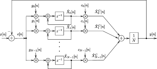
An extension of the FA is an observer-based algorithm that can be used for the analysis of non-coherently sampled periodic signals as well as for order tracking. To achieve this, only the so-called basis vectors of the DFT are to be substituted by another complex exponentials having the same fundamental frequency as the input signal. However, the appropriate basis function set calls for the estimation of the fundamental frequency of the input signal. The extended observer, called Adaptive Fourier Analyzer (AFA), is able to estimate both the fundamental frequency and the spectrum of the input signal simultaneously, as shown in Fig. 2.
Fig.2. The structure of the observer-based Adaptive Fourier Analyzer (AFA). The resonator positions are shown by colored dots, with the corresponding amplitude estimates having the same color. In the illustration the input signal contains 1st, 3rd, 5th, and 7th harmonics; the corresponding colors are red, green, purple, and orange, respectively.
AFA has been first proposed in [3], as an application of nonlinear signal processing. Later the
observer has been extended for the error-free reconstruction of periodic signals of linear,
logarithmic as well as hyperbolic time-frequency functions [4]. The paper introduces the design of
the AFA in detail, provides tips and tricks for the practical implementation,
addresses the stability issues, and compares it to other methods. The provided
AFA implementation [afa.m] can be regarded as reference implementation,
containing all aspects discussed in the paper.
The MATLAB codes provided below help you to get more familiar with the AFA algorithm.
Use the graphical user interface [afagui.m] to experiment with AFA.
Should you wish to tweak more parameters, a command line option is also provided [afa.m] with
a set of auxiliary files (input signal generators and a plotter).
The MATLAB codes can be downloaded in a zip file from here.
afagui.m]. You can select from a set of input signals and configure the input noise level. You can also
set some parameters of the AFA (signal model (constant frequency, linearly, logarithmically, hyperbolically changing frequency), initial
frequency estimate, frequency adaptation gain). Press RUN to see the results. The interface is shown in Fig. 3.
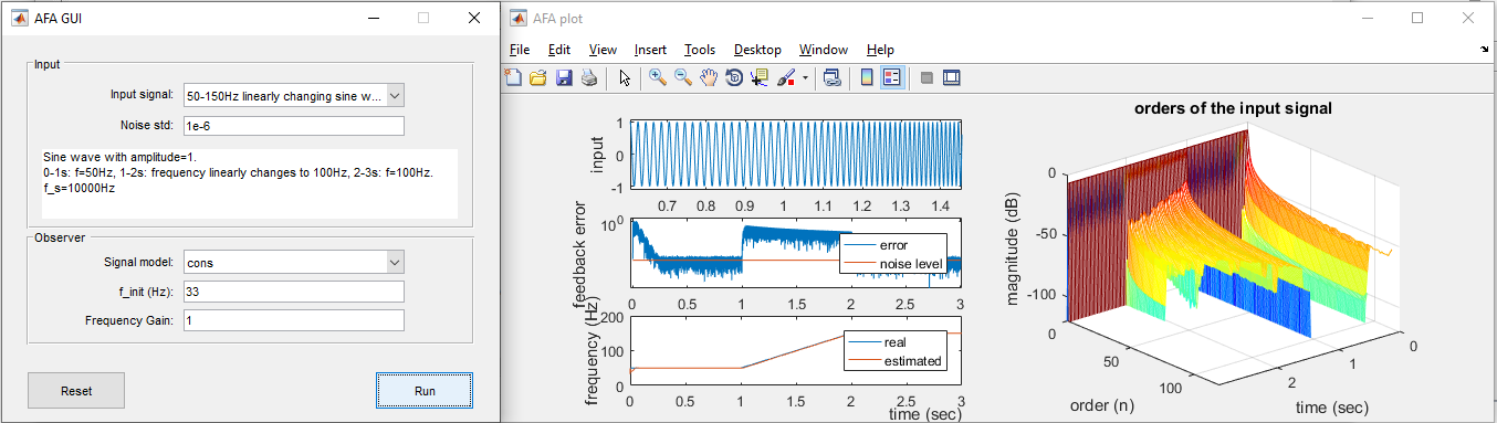
Fig.3. The Graphical User Interface with the plotted input and output signals
The sampling frequency is set to fs = 10 kHz in all cases.
in_50.m], f = 50 Hz. The duration of the signal is 3 seconds.
in_50_150_lin.m]. The duration of the signal is 3 seconds.
In the first second the frequency is 50 Hz, which linearly increases to 150 Hz between 1 sec and 2 sec. In the last second the frequency is 150 Hz.
in_50_150_log.m]. The duration of the signal is 3 seconds.
In the first second the frequency is 50 Hz, which logarithmically increases to 150 Hz between 1 sec and 2 sec. In the last second the frequency is 150 Hz.
in_50_150_hyp.m]. The duration of the signal is 3 seconds.
In the first second the frequency is 50 Hz, which hyperbolically increases to 150 Hz between 1 sec and 2 sec. In the last second the frequency is 150 Hz.
rect_50_150_lin.m]. The duration of the signal is 3 seconds.
In the first second the fundamental frequency is 50 Hz, which linearly increases to 150 Hz between 1 sec and 2 sec. In the last second the frequency is 150 Hz.
This is the excitation signal used in the paper as the first exapmle.
rect_50_150_lin_noise.m]. The duration of the signal is 3 seconds.
In the first second the fundamental frequency is 50 Hz, which linearly increases to 150 Hz between 1 sec and 2 sec. In the last second the frequency is 150 Hz.
The signal is burdened with Gaussian noise with SNR of 40 dB. This is the excitation signal used in the paper as the second exapmle.
mix_50_100_150.m]. The duration of the signal is 3 seconds.
In the first second the signal is a sine wave of 50 Hz with amplitude of 1, followed by a square wave of 100 Hz with amplitude of 1.5 between 1 sec and 2 sec,
and finally a triangular wave of 150 Hz with amplitude of 2 in the last second.
All signal generator scripts produce their output to the current workspace. The outputs contain the signal itself (variable in),
and other auxiliary variables to aid the presentation of the results in AFAplot.
AFAplot.m]. Plots the input signal and the estimated frequency and spectrum (see the right hand side of Fig. 3).
For sake of convenience, a plotter is provided, which plots the input signal and the output of the AFA. The plotter uses the variables produced by the signal generators along with the output of the AFA, using the name convention shown in section Usage.
afa.m].The AFA calculates the frequency estimate,
the orders, and the feedback error of an input signal.
See help afa for more details.
Select a signal generator (e.g. the linearly sweeping sine wave [in_50_150_lin.m]). Type:
in_50_150_lin
[frequency, fb_error, orders]=afa(in);
AFAplot
An example with more input parameters for the AFA (see help afa for more details):
in_50_150_log
[frequency, fb_error, orders] = afa(in, 'log', 1, 0.01, 256);
AFAplot
Note: If you want to use the provided AFAplot program, you must use the names shown in the examples as output parameters for AFA.